Depth-first traversal or Depth-first Search is an algorithm to look at all the vertices of a graph or tree data structure. Here we will study what depth-first search in python is, understand how it works with its bfs algorithm, implementation with python code, and the corresponding output to it.
What is Depth First Search?
What do we do once have to solve a maze? We tend to take a route, keep going until we discover a dead end. When touching the dead end, we again come back and keep coming back till we see a path we didn't attempt before. Take that new route. Once more keep going until we discover a dead end. Take a come back again… This is exactly how Depth-First Search works.
The Depth-First Search is a recursive algorithm that uses the concept of backtracking. It involves thorough searches of all the nodes by going ahead if potential, else by backtracking. Here, the word backtrack means once you are moving forward and there are not any more nodes along the present path, you progress backward on an equivalent path to seek out nodes to traverse. All the nodes are progressing to be visited on the current path until all the unvisited nodes are traversed after which subsequent paths are going to be selected.
DFS Algorithm
Before learning the python code for Depth-First and its output, let us go through the algorithm it follows for the same. The recursive method of the Depth-First Search algorithm is implemented using stack. A standard Depth-First Search implementation puts every vertex of the graph into one in all 2 categories: 1) Visited 2) Not Visited. The only purpose of this algorithm is to visit all the vertex of the graph avoiding cycles.
The DSF algorithm follows as:
- We will start by putting any one of the graph's vertex on top of the stack.
- After that take the top item of the stack and add it to the visited list of the vertex.
- Next, create a list of that adjacent node of the vertex. Add the ones which aren't in the visited list of vertexes to the top of the stack.
- Lastly, keep repeating steps 2 and 3 until the stack is empty.
DFS pseudocode
The pseudocode for Depth-First Search in python goes as below: In the init() function, notice that we run the DFS function on every node because many times, a graph may contain two different disconnected part and therefore to make sure that we have visited every vertex, we can also run the DFS algorithm at every node.
DFS(G, u)
u.visited = true
for each v ∈ G.Adj[u]
if v.visited == false
DFS(G,v)
init() {
For each u ∈ G
u.visited = false
For each u ∈ G
DFS(G, u)
}
DFS Implementation in Python (Source Code)
Now, knowing the algorithm to apply the Depth-First Search implementation in python, we will see how the source code of the program works.
Consider the following graph which is implemented in the code below:
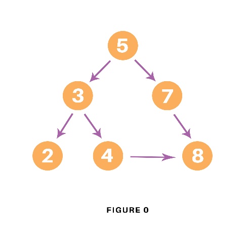
graph = {
  '5' : ['3','7'],
  '3' : ['2', '4'],
  '7' : ['8'],
  '2' : [],
  '4' : ['8'],
  '8' : []
}

visited = set() # Set to keep track of visited nodes of graph.

def dfs(visited, graph, node):  #function for dfs
    if node not in visited:
        print (node)
        visited.add(node)
        for neighbour in graph[node]:
            dfs(visited, graph, neighbour)


print("Following is the Depth-First Search")
dfs(visited, graph, '5')
In the above code, first, we will create the graph for which we will use the depth-first search. After creation, we will create a set for storing the value of the visited nodes to keep track of the visited nodes of the graph.
After the above process, we will declare a function with the parameters as visited nodes, the graph itself and the node respectively. And inside the function, we will check whether any node of the graph is visited or not using the “if” condition. If not, then we will print the node and add it to the visited set of nodes.
Then we will go to the neighboring node of the graph and again call the DFS function to use the neighbor parameter.
At last, we will run the driver code which prints the final result of DFS by calling the DFS the first time with the starting vertex of the graph.
Output
The output of the above code is as follow:
Following is the Depth-First Search
5 3 2 4 8 7
Time Complexity
The time complexity of the Depth-First Search algorithm is represented within the sort of O(V + E), where V is that the number of nodes and E is that the number of edges.
The space complexity of the algorithm is O(V).
Applications
Depth-First Search Algorithm has a wide range of applications for practical purposes. Some of them are as discussed below:
- For finding the strongly connected components of the graph
- For finding the path
- To test if the graph is bipartite
- For detecting cycles in a graph
- Topological Sorting
- Solving the puzzle with only one solution.
- Network Analysis
- Mapping Routes
- Scheduling a problem
Conclusion
Hence, Depth-First Search is used to traverse the graph or tree. By understanding this article, you will be able to implement Depth-First Search in python for traversing connected components and find the path.
They are two of the most important topics that any new python programmer should definitely learn about. Here we will study what breadth-first search in python is, understand how it works with its algorithm, implementation with python code, and the corresponding output to it. Also, we will find out the application and uses of breadth-first search in the real world.
What is Breadth-First Search?
As discussed earlier, Breadth-First Search (BFS) is an algorithm used for traversing graphs or trees. Traversing means visiting each node of the graph. Breadth-First Search is a recursive algorithm to search all the vertices of a graph or a tree. BFS in python can be implemented by using data structures like a dictionary and lists. Breadth-First Search in tree and graph is almost the same. The only difference is that the graph may contain cycles, so we may traverse to the same node again.
BFS Algorithm
Before learning the python code for Breadth-First and its output, let us go through the algorithm it follows for the same. We can take the example of Rubik’s Cube for the instance. Rubik’s Cube is seen as searching for a path to convert it from a full mess of colors to a single color. So comparing the Rubik’s Cube to the graph, we can say that the possible state of the cube is corresponding to the nodes of the graph and the possible actions of the cube is corresponding to the edges of the graph.
As breadth-first search is the process of traversing each node of the graph, a standard BFS algorithm traverses each vertex of the graph into two parts: 1) Visited 2) Not Visited. So, the purpose of the algorithm is to visit all the vertex while avoiding cycles.
BFS starts from a node, then it checks all the nodes at distance one from the beginning node, then it checks all the nodes at distance two, and so on. So as to recollect the nodes to be visited, BFS uses a queue.
The steps of the algorithm work as follow:
- Start by putting any one of the graph’s vertices at the back of the queue.
- Now take the front item of the queue and add it to the visited list.
- Create a list of that vertex's adjacent nodes. Add those which are not within the visited list to the rear of the queue.
- Keep continuing steps two and three till the queue is empty.
Many times, a graph may contain two different disconnected parts and therefore to make sure that we have visited every vertex, we can also run the BFS algorithm at every node.
BFS pseudocode
The pseudocode for BFS in python goes as below:
create a queue Q
mark v as visited and put v into Q
while Q is non-empty
remove the head u of Q
mark and enqueue all (unvisited) neighbors of u
BFS implementation in Python (Source Code)
Now, we will see how the source code of the program for implementing breadth first search in python.
Consider the following graph which is implemented in the code below:

graph = {
  '5' : ['3','7'],
  '3' : ['2', '4'],
  '7' : ['8'],
  '2' : [],
  '4' : ['8'],
  '8' : []
}

visited = [] # List for visited nodes.
queue = []     #Initialize a queue

def bfs(visited, graph, node): #function for BFS
  visited.append(node)
  queue.append(node)

  while queue:          # Creating loop to visit each node
    m = queue.pop(0)
    print (m, end = " ")

    for neighbour in graph[m]:
      if neighbour not in visited:
        visited.append(neighbour)
        queue.append(neighbour)


print("Following is the Breadth-First Search")
bfs(visited, graph, '5')    # function calling
In the above code, first, we will create the graph for which we will use the breadth-first search. After creation, we will create two lists, one to store the visited node of the graph and another one for storing the nodes in the queue.
After the above process, we will declare a function with the parameters as visited nodes, the graph itself and the node respectively. And inside a function, we will keep appending the visited and queue lists.
Then we will run the while loop for the queue for visiting the nodes and then will remove the same node and print it as it is visited.
At last, we will run the for loop to check the not visited nodes and then append the same from the visited and queue list.
As the driver code, we will call the user to define the bfs function with the first node we wish to visit.
Output
The output of the above code will be as follow:
Following is the Breadth-First Search
5 3 7 2 4 8
Time Complexity
The time complexity of the Breadth first Search algorithm is in the form of O(V+E), where V is the representation of the number of nodes and E is the number of edges.
Also, the space complexity of the BFS algorithm is O(V).
Applications
Breadth-first Search Algorithm has a wide range of applications in the real-world. Some of them are as discussed below:
- In GPS navigation, it helps in finding the shortest path available from one point to another.
- In pathfinding algorithms
- Cycle detection in an undirected graph
- In minimum spanning tree
- To build index by search index
- In Ford-Fulkerson algorithm to find maximum flow in a network.
Conclusion
If you have a good understanding of core python concepts and with the help of what you read today, you can now easily implement breadth first search in python. I hope this article clearly explained how this algorithm works.
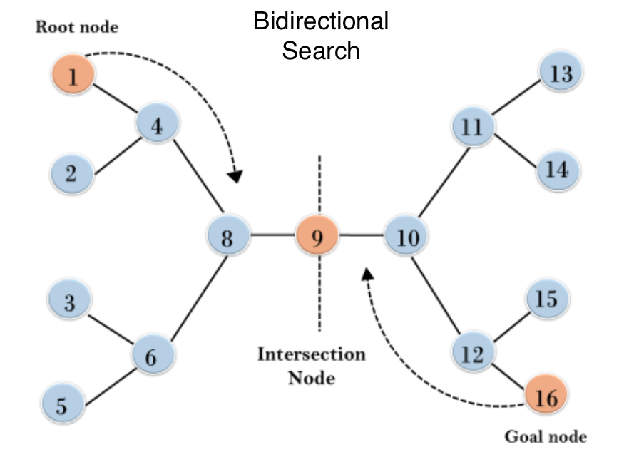
Bidirectional search
Bidirectional search is a graph search algorithm that finds the shortest path from a source vertex to a goal vertex.
In implementing bidirectional search in Python, the graph search can either be:
- Forward search from the source to the goal vertex.
- Backward search from the goal to the source vertex.
The intersection of both forward and backward graphs indicates the end of the search, as displayed below.
Advantages and disadvantages of bidirectional search in Python
| Advantage | Disadvantage |
|---|
| 1. Less time consuming as the shortest path length is used for the search. | The goal node has to be known before the search can be done simultaneously in both directions. |
When is it possible to use bidirectional search in Python?
The bidirectional approach can be used:
- When the branching factor for the forward and reverse direction is the same.
- When both the source and goal vertices are specified and distinct from each other.
Bidirectional search implementation in Python
Below is an implementation of bidirectional search in Python using BFS:
Python Code:
class adjacent_Node:
def __init__(self, v):
self.vertex = v
self.next = None
class bidirectional_Search:
def __init__(self, vertices):
self.vertices = vertices
self.graph = [None] * self.vertices
self.source_queue = list()
self.last_node_queue = list()
self.source_visited = [False] * self.vertices
self.last_node_visited = [False] * self.vertices
self.source_parent = [None] * self.vertices
self.last_node_parent = [None] * self.vertices
def AddEdge(self, source, last_node):
node = adjacent_Node(last_node)
node.next = self.graph[source]
self.graph[source] = node
node = adjacent_Node(source)
node.next = self.graph[last_node]
self.graph[last_node] = node
def breadth_fs(self, direction = 'forward'):
if direction == 'forward':
current = self.source_queue.pop(0)
connected_node = self.graph[current]
while connected_node:
vertex = connected_node.vertex
if not self.source_visited[vertex]:
self.source_queue.append(vertex)
self.source_visited[vertex] = True
self.source_parent[vertex] = current
connected_node = connected_node.next
else:
current = self.last_node_queue.pop(0)
connected_node = self.graph[current]
while connected_node:
vertex = connected_node.vertex
if not self.last_node_visited[vertex]:
self.last_node_queue.append(vertex)
self.last_node_visited[vertex] = True
self.last_node_parent[vertex] = current
connected_node = connected_node.next
def is_intersecting(self):
#
for i in range(self.vertices):
if (self.source_visited[i] and
self.last_node_visited[i]):
return i
return -1
def path_st(self, intersecting_node,
source, last_node):
path = list()
path.append(intersecting_node)
i = intersecting_node
while i != source:
path.append(self.source_parent[i])
i = self.source_parent[i]
path = path[::-1]
i = intersecting_node
while i != last_node:
path.append(self.last_node_parent[i])
i = self.last_node_parent[i]
print("*****Path*****")
path = list(map(str, path))
print(' '.join(path))
def bidirectional_search(self, source, last_node):
self.source_queue.append(source)
self.source_visited[source] = True
self.source_parent[source] = -1
self.last_node_queue.append(last_node)
self.last_node_visited[last_node] = True
self.last_node_parent[last_node] = -1
while self.source_queue and self.last_node_queue:
self.breadth_fs(direction = 'forward')
self.breadth_fs(direction = 'backward')
intersecting_node = self.is_intersecting()
if intersecting_node != -1:
print("Path exists between {} and {}".format(source, last_node))
print("Intersection at : {}".format(intersecting_node))
self.path_st(intersecting_node,
source, last_node)
exit(0)
return -1
if __name__ == '__main__':
n = 17
source = 1
last_node = 16
my_Graph = bidirectional_Search(n)
my_Graph.AddEdge(1, 4)
my_Graph.AddEdge(2, 4)
my_Graph.AddEdge(3, 6)
my_Graph.AddEdge(5, 6)
my_Graph.AddEdge(4, 8)
my_Graph.AddEdge(6, 8)
my_Graph.AddEdge(8, 9)
my_Graph.AddEdge(9, 10)
my_Graph.AddEdge(10, 11)
my_Graph.AddEdge(11, 13)
my_Graph.AddEdge(11, 14)
my_Graph.AddEdge(10, 12)
my_Graph.AddEdge(12, 15)
my_Graph.AddEdge(12, 16)
out = my_Graph.bidirectional_search(source, last_node)
if out == -1:
print("No path between {} and {}".format(source, last_node))
Output:


